Diagnosing Java Performance Problems with the GC Log Analyzer
Although the Java platform simplifies many aspects of software development, it introduces side effects of its runtime environment and memory models that can negatively affect runtime performance. Some performance concerns include the following:
-
System pauses during garbage collection (GC)
-
Warmup delays for just-in-time compilation
-
Response latencies
Once you have identified performance problems, you can perform root-cause analysis to determine the exact cause of the problem. You can perform root-cause analysis with unit and system tests but another option is to analyze the GC log.
This article describes the following:
-
How to create a GC log
-
How to view the log data in the GC Log Analyzer tool
-
How to interpret log analyzer metrics and visual graphs to resolve common Java performance problems.
It’s important to note that the GC Log Analyzer can help identify a wide range of problems, from common to uncommon and from severe to trivial, which means choosing which graphs to look at in order to identify particular problems is purely a subjective task which changes from person to person. The information covered in this guide is meant to give you only a general idea of how to identify the most common and severe problems, using real-world examples.
Generating GC Logs
To begin analysis of a poorly performing application, you must generate a GC log. Start your application with an additional parameter to begin generating the log file:
java -Xlog:gc:<filename> -jar <application.jar>
The -Xlog:gc:<filename> parameter tells the Java Virtual Machine (JVM) to log garbage collection information to the file you specify.
Although the log generator supports many options, the above is enough to get started. You can learn more about GC log output options from the Unified Logging documentation.
Run your application under the same stress as your live application if possible. If not, you may have to simulate typical application conditions so that you duplicate the problematic behavior. Once you have a sufficient amount of log data, you are ready to view the logs with the GC Log Analyzer.
Downloading and Running the Analyzer
To run the GC Log Analyzer:
-
Download GC Log Analyzer.
-
Open GC Log Analyzer using the following command:
java -jar GCLogAnalyzer2.jar <filename.log>
The <filename> argument is optional and opens the specified log file in GC Log Analyzer at startup. Log files can also be opened once GC Log analyzer is running using File > Open File or by simply dragging and dropping a log file into the GC Log Analyzer application window.
Understanding the Analyzer
The log analyzer has many analytical and display options. You can learn more details about these options from the Using the GC Log Analyzer documentation. For this article, we will cover some of the highlights and most helpful graphs.
The log analyzer helps you to understand an application’s performance, memory usage, pauses, CPU usage, and even object allocation rates. As we investigate the analyzer, we will use a sample log file. Using this log, we will look at important screens within the UI that can help us understand the application’s performance.
When looking at the analyzer graphs, it’s easy to feel overwhelmed with information. The GC logs can be quite verbose. It’s best to keep things simple. We’ll look at the following items in order:
-
General Information
-
GC Time (percent)
-
GC Count
-
Heap Collected
-
Load Average
-
Live Set
General Information
The following image outlines the main parts of the GC Log Analyzer application.
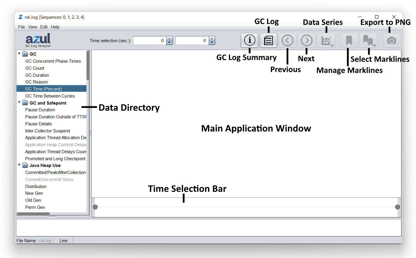
The first screen to look at is the basic information screen. Click ![]() at the top of the log analyzer screen.
at the top of the log analyzer screen.
The general information screen shows basic static information about your system such as the following:
-
Host Name
-
CPU Count
-
Total RAM
-
JVM Arguments
Along the left side of the analyzer screen is the list of all graphs provided by the tool, in the data directory. For the purpose of this guide, we will only be looking at a few of these graphs.
Whenever you click on a graph, the graph’s time selection bar will appear below the graph itself. This is a tool for analyzing a particular portion of the graph. You can refine or expand the view by dragging the dots left or right.

Looking at the Graphs
The GC Log Analyzer contains a lot of data and can seem overwhelming. It’s important to familiarize yourself with which graphs can indicate which problems. The following graphs were chosen for this example as they are commonly used to identify particular common problems. The graphs in the following sections displaying problematic behavior were obtained using an application simulator. All of the following graphs are from the same system using the same bad system setup.
The initial bad setup has the following problems:
-
Heaps are too small - 8GB
-
Elastic heap set to true
-
Large amount of reference data loaded - 5GB
-
No garbage collection after reference data is loaded
-
Too short rampup
-
Too high transaction rates - 4 threads with 200 transactions/second each
GC > GC Time (Percent)
Click GC > GC Time (Percent) to see the percent of time that the garbage collector threads are running along the Y axis, over time along the X axis.
The following graph shows collector threads running 100% of the time very frequently. Any spike above 30% should be investigated. This is a clear indication of a problem. Because the GC is running frequently and for long amounts of time, the application may be suffering from a lack of heap memory size.
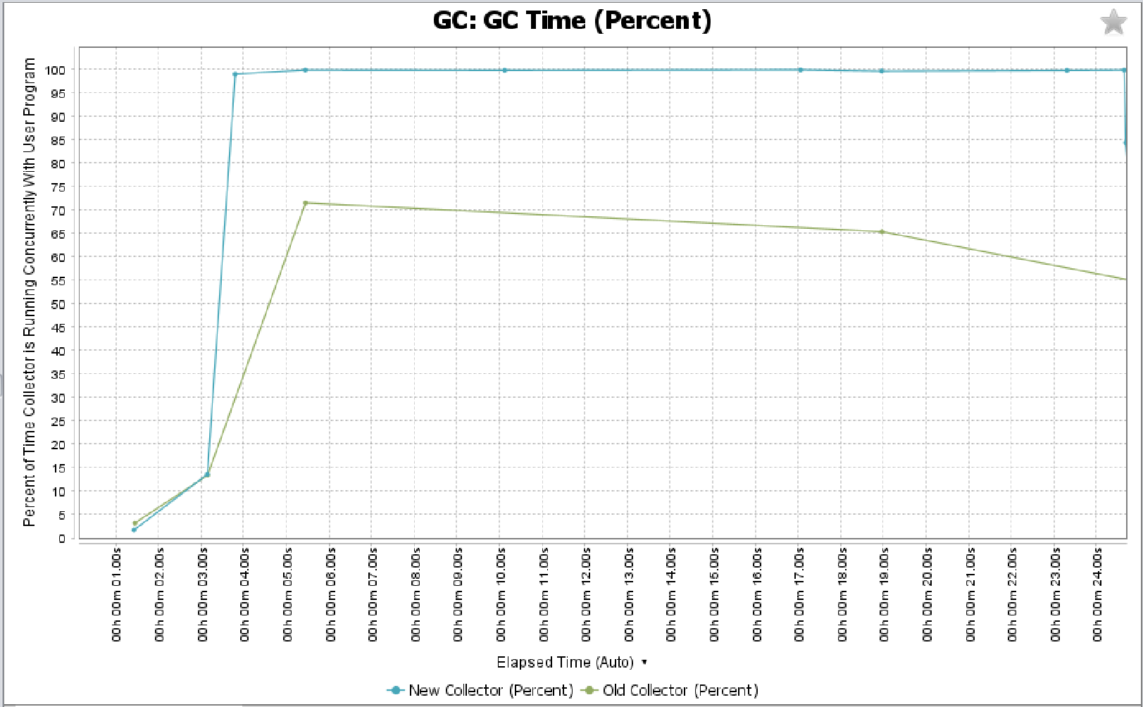
The next graph shows a healthy GC Time graph:
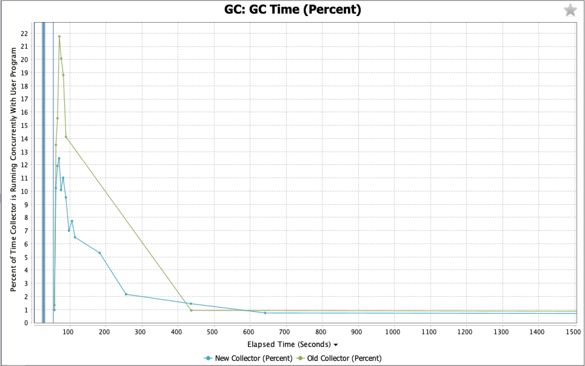
GC > GC Count
Click GC > GC Count to see the accumulated count of GC cycles over the lifetime of the application. In the following graph, focus on the "New GC Count" line (blue). Look for periods where the new GC count rises quickly.
Calculate the number of cycles per minute. Take two points on the graph, and calculate the time differential and the GC count differential. We want to calculate cycles per minute. You should investigate anything over 10 cycles/minute. Anything over 20 cycles/minute is a serious concern.
In the above graph, let’s look at the 1-minute interval from 30 seconds to 1 minute 30 seconds. If you hover the mouse over the graph, the analyzer will show you the exact time and GC count. Using the above graph, we do the following calculation:
 72 cycles - 17 cycles = 55 cycles
72 cycles/1 min = 55 cycles/min
The graph above shows that the GC is running 55 times a minute. This is a serious cause for concern.
The following graph shows a healthy GC count graph. When we use the same method to calculate GC cycles, using a 10 minute interval, we can see that the GC is running just 0.2 times a minute.
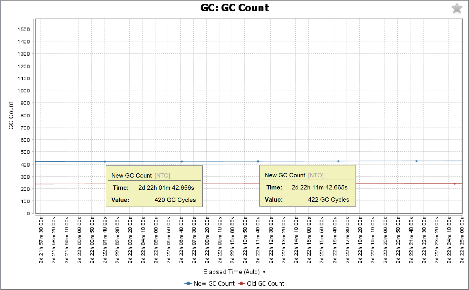
 422 cycles – 420 cycles = 2 cycles
2 cycles/10 min = 0.2 cycles/min
Java Heap > Garbage Collected
click Java Heap > Garbage Collected to see the amount of memory reclaimed by the garbage collector for both "newGen" and "oldGen" memory. The more garbage collected per cycle, the better.
Watch for dramatic drops in the amount of garbage collected per collection cycle. This is particularly troublesome if you also notice cycle frequency increases, too. Typically, a healthy graph will show newGen cycles reclaim at least 10x than oldGen cycles.
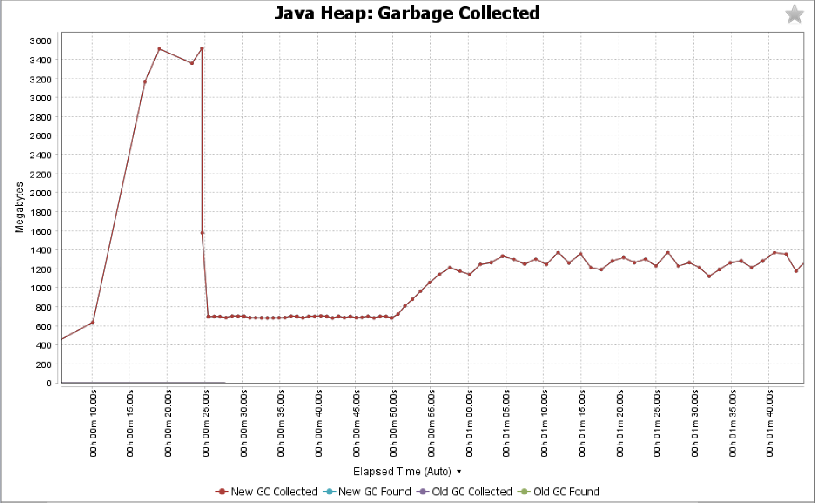
The following graph shows an unhealthy Java Heap graph.
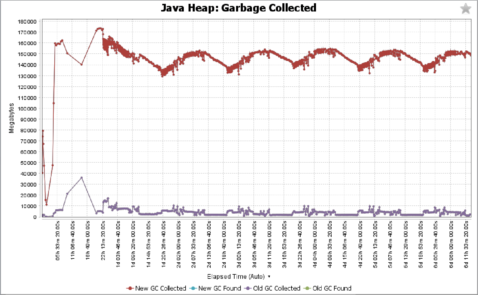
You can compare the above graph to the below graph, showing a healthy Java Heap graph.
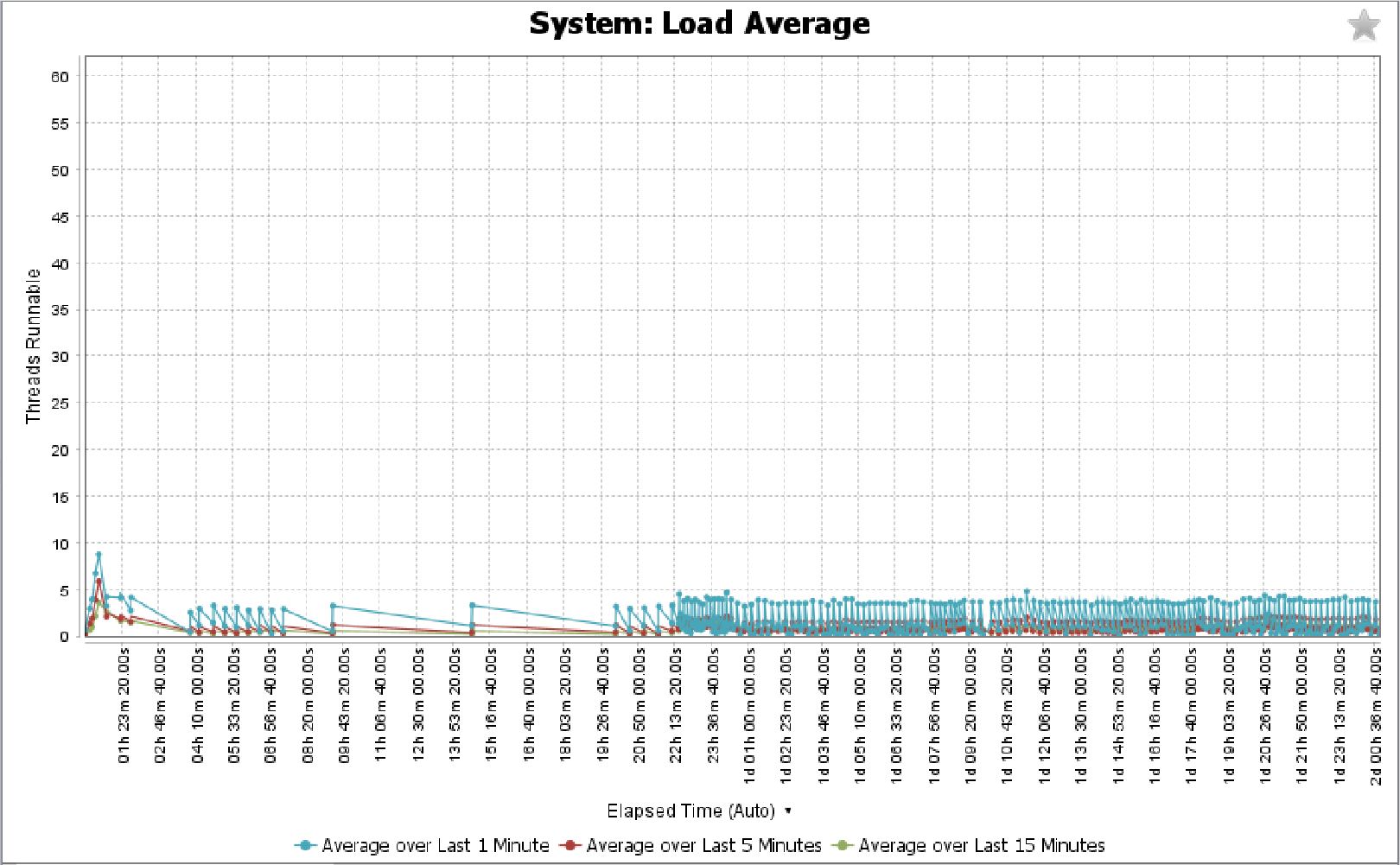
System > Load Average
Click System > Load Average to display the thread count over time as the application runs. One sign of memory pressure is a thread count spike that is greater than the number of cores.
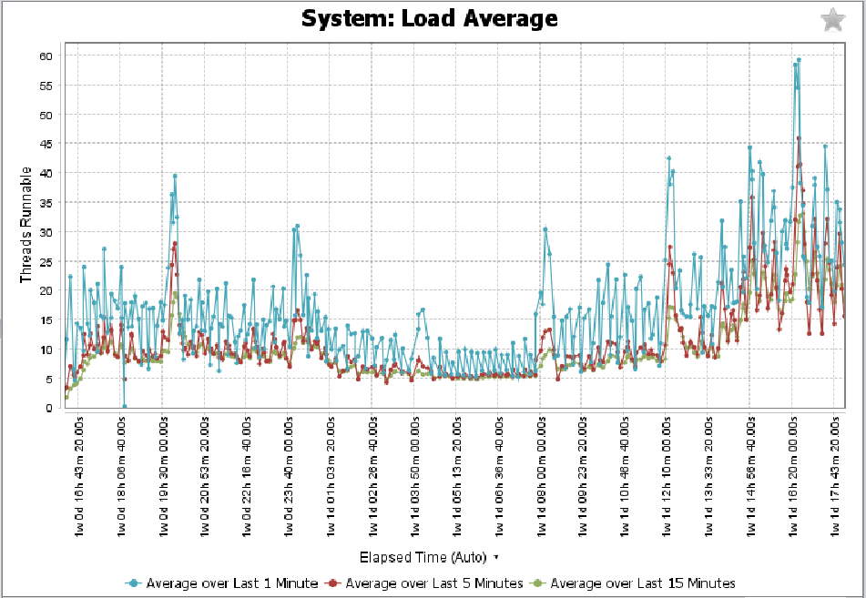
For example, the following graph, from a machine with 8 cores and 16 threads, shows frequent jumps above 20 system threads, all the way up to 60 system threads, which suggests low memory.
The following graph, from the same machine with 8 cores and 16 threads, shows a healthy Load Average graph, showing a steady average load under 5 threads.
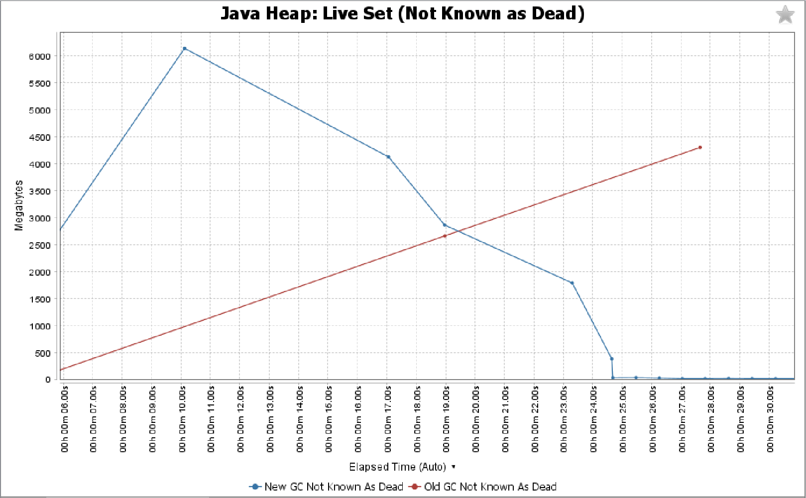
Java Heap > Live Set
Click Java Heap > Live Set (either Known Live or Not Known as Dead) to show how big the objects were during garbage collection cycles. This set of graphs is only an estimate of object size. The "Known Live" graph represents an underestimate while the "Not Known as Dead" graph represents an overestimate. Old heap garbage collection is more stable than new heap garbage collection.
You know from the system configuration that reference data is being loaded at the beginning. With this in mind, the following unhealthy graph shows that too much reference data is being loaded at system startup, causing system instability. Furthermore, you can see that old heap garbage collection stops entirely after just 28 seconds.
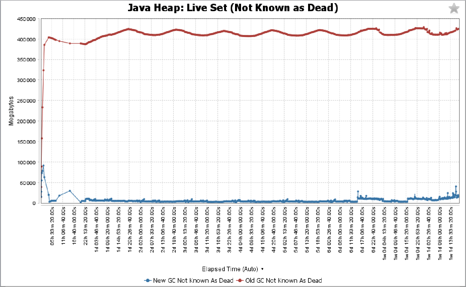
The following healthy graph shows the same initial loading of reference data, yet old heap garbage collection continues to an eventually stable state.
Conclusions
The GC Log Analyzer is an important tool for understanding application and JVM performance. Although the tool has much more functionality, you can gain significant awareness of your application performance by investigating just a few major graphs and metrics. Here is a brief review of the graphs covered in this guide and why they are important:
-
GC > GC Time (percent) - Even if all else is perfect, irregularities and too high of a value may hint towards a scalability limitation.
-
GC > GC Count - A high number of garbage collection cycles indicates a serious problem.
-
Java Heap > Garbage Collected - Should be nice and regular newGen and fairly infrequent oldGen.
-
System > Load Average - Check if your CPU is being overloaded.
-
Java Heap > Live Set - Too big of a live set with too little room to spare.
In the examples shown in this article, GC cycle times were frequent and often ran at 100% capacity. This is indicative of significant memory pressure. Although system memory is significantly higher than application memory, we might suspect that the heap size is too small. One of the resolutions includes increasing heap size.